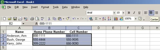
Below is the screen of a typical Excel document.
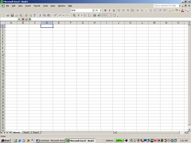
The power of Excel is great, but we are going to look at the basics of how it can make our lives easier by knowing and understanding the fundamentals of Excel.
Notice that Excel is basically a table with multiple columns and rows. The columns are labeled A, B, C, etc. while the rows are numbered 1, 2, 3, etc. (There are a total of 256 columns and 65536 rows, so you shouldn’t run out of space.) Each space is called a cell and each cell has a name that corresponds to its letter and number space. Thus, the top left cell would be called A1. The cell below it would be A2 while the cell to the right of A1 would be B1.
Look at the spreadsheet below.
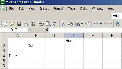
Tell which cell each of the following is in.
Tiger is in cell _____. Cat is in cell ____. Horse is in cell _____.
You should have noticed that Tiger is in cell A4, Cat is in cell B2, and Horse is in cell D1.
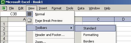
Before we go any further, it is wise that we make sure our screen has most of the common toolbars that are available in Excel so that we can do things quickly and not have to search through the Menu bar for the items. To display the typical toolbars, you will want to go the View menu in the Menu bar. Scroll down to Toolbars and highlight the Standards button. Go back and also highlight the Formatting button. Look below for a picture representation.
Now that we have taken care of creating quick shortcuts to the common features of Excel, let’s take a look at some things Excel can do.
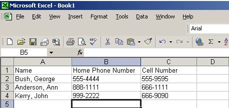
Let’s say we want to make a list of our friends’ phone numbers by using Excel.
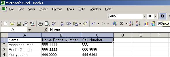
First, we would click our mouse into cell A1 and title it Name. To move to cell B1, we can use our mouse and click in cell B1 or we can hit the Tab button or the right arrow button. Hitting return (Enter) will move the cursor to A2, which is not a problem since we can use the mouse to click in B1. In B1, enter “Home Phone Number.” More than likely when you finished entering this information, you noticed that your information looked like it was in cell C1 like below.
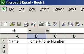
Don’t worry, for it doesn’t affect C1 at all. We simply need to make column B wider. To do so, you have two options. First, click in cell B1 and then go to the Menu bar and click on Format. Select Column and then Autofit Selection. This feature will make the column the exact length it needs to be. The easier option is to move your cursor between the letters B and C. Your screen should look like below.
Click and drag column B to the right as far as you would like it to go.
Now click in cell C1 and enter “Cell Number.” Again, widen column C so everything fits nicely in the column. Now try to enter the information that is below into each of the appropriate cells.
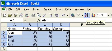
You may have noticed that the names are not in alphabetical order. So, let’s fix it. No, we don’t have to retype them. All we have to do is click (and hold) in cell A2 where our names start and drag our mouse over to cell C4 so that we have highlighted all of the information. Your screen should look like the picture below.
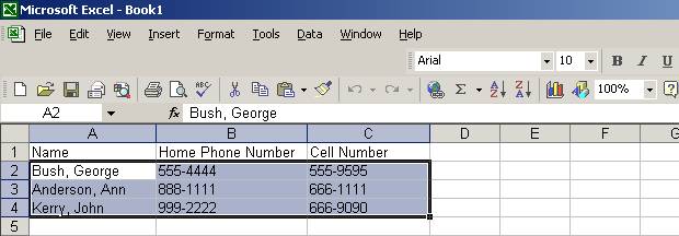
Notice that we started by highlighting the names we want to put in alphabetical order, but also highlighted the other information that went with it so that when we sort the information, we will keep the people’s phone numbers and cell numbers with the correct name.
Now move your cursor over top of the toolbar button ![]() which sorts
information in ascending order. (If you
wanted to sort in descending order, you would click on the toolbar button
which sorts
information in ascending order. (If you
wanted to sort in descending order, you would click on the toolbar button ![]() .)
.)
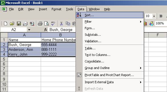
If you can’t find the ![]() toolbar button, you can go to the Menu bar and
click on Data and then the Sort button like below.
toolbar button, you can go to the Menu bar and
click on Data and then the Sort button like below.
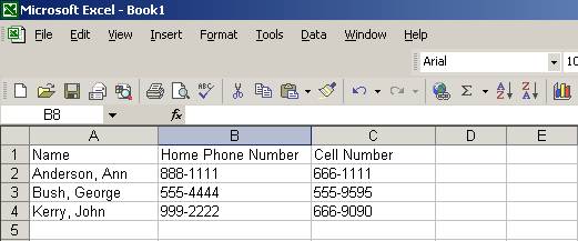
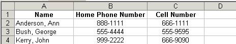
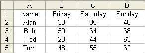
Your screen should now look like the screen below.
The information above is good, but let’s fix it so that it looks a little neater.
It would be nice to make the main information in row 1 bold and in the center of each column. To make the information bold we highlight everything in row 1 by clicking in cell A1 and dragging over to cell C1.
Once you have highlighted cells A1 through C1, move over to
the toolbar button ![]() and click on it. Notice that in the example above, the
and click on it. Notice that in the example above, the ![]() button is located in the right hand corner.
button is located in the right hand corner.
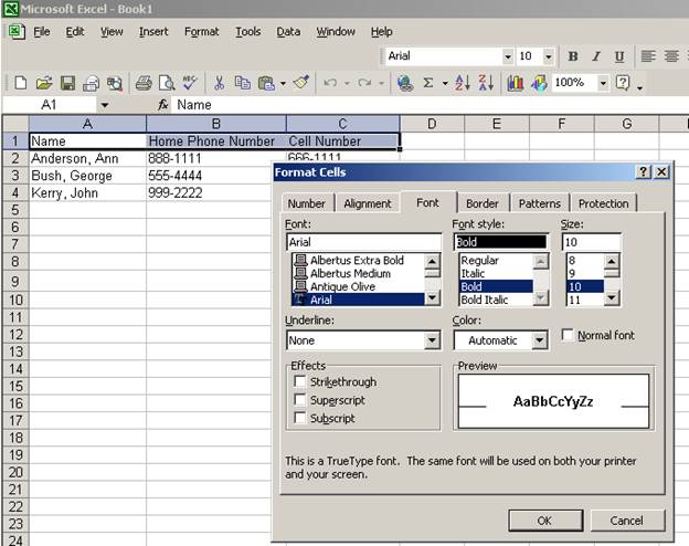
If you do not have this icon showing, you can go to the Format button and click on cells. You then will move over to the Font tab and click on the word Bold and then click OK. Look below.
(We will discuss more about the Format Cells button later in the chapter.)
To center the information, we will again highlight cells A1
through C1 and click on the ![]() button which is located
in the
button which is located
in the ![]() section of the screen. If you cannot find it in the toolbar, you can
center the information by again going to the Format button and clicking on
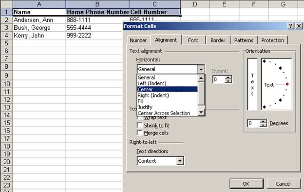
Cells. This time you will click on the
Alignment tab and pick Center from the menu under Horizontal. Click OK and the information will be centered.
section of the screen. If you cannot find it in the toolbar, you can
center the information by again going to the Format button and clicking on
Cells. This time you will click on the
Alignment tab and pick Center from the menu under Horizontal. Click OK and the information will be centered.
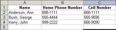
Now our information should appear like below.
We might want to center all of the numbers in column B and
column C to make it look a little better.
To do so, highlight everything in column B and C and then click on the
center icon ![]() .
.
Now our screen looks like below.
If you like, you can center all of the names, too.
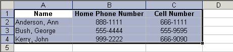
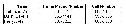
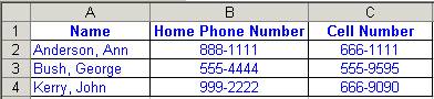
At this point, we would want to print out our list of names and numbers. If we print the way it is now, it will appear without any lines and look like below.
If we want to put it in table form, we can highlight everything by clicking in cell A1 and dragging our cursor over to cell C4. Everything should be highlighted like below.
Now we will go to the toolbar and select the borders icon.
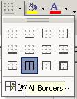
To put a border around the information, we will choose the ![]() icon, which is highlighted
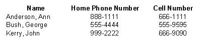
in the picture above. Now when we print,
our information will appear like that below.
icon, which is highlighted
in the picture above. Now when we print,
our information will appear like that below.
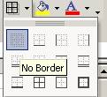
If you don’t like the way this looks and you want it without any border, simply highlight the information again, click on the borders icon and pick the icon shown below which is the no border icon.
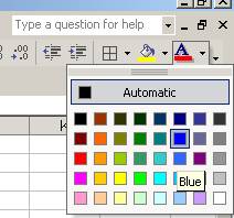
If we want to make the information colorful, we can either color in the cells or change the font to any color we like. Let’s color our font blue and make each cell yellow.
To color the font blue, we will highlight all cells (A1 –
C4) and then go over to the icon that looks like ![]() . Click on this icon and select the color
blue.
. Click on this icon and select the color
blue.
Now our spreadsheet looks like below.
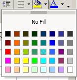
To make each cell yellow, we will highlight all of the cells and go to the ![]() icon and select the color yellow.
icon and select the color yellow.
Now, our screen should look like below.
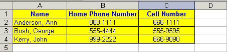
If we want to change the color of the font or the cells, we simply go back to the icon and select a different color or pick “No Fill” if we wish for the cells to not have any background color.
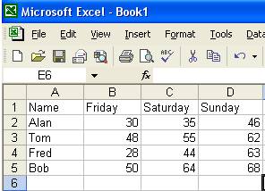
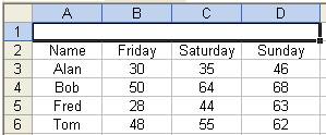
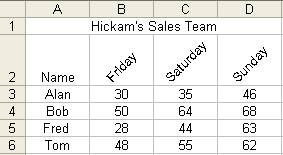
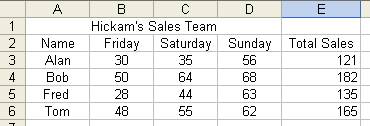
Let’s turn our attention to another more complex project. Let’s say that we run a small business on the weekend which has four employees. Put the following information in like it appears below.
Before we learn anything new, let’s put all the names in alphabetical order and center all of the information. Remember that to put the names in alphabetical order, you highlight A2 (where the first name appears) and drag down over all the names and out to D5 so that it carries the information with it.
Now hit the ![]() button to put the names in alphabetical
order. Now to center all of the
information, we must highlight everything including all of row 1 and hit the
button to put the names in alphabetical
order. Now to center all of the
information, we must highlight everything including all of row 1 and hit the ![]() button to center the information. Now your screen should look like below.
button to center the information. Now your screen should look like below.
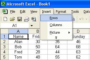
One thing I might want to do to this information is add a row above the A, B, C, and D column and put some title to it like “ Hickam’s Team Sales.” To add a row, we must click our cursor in any of the cells in row 1 and then go to the Menu bar and click on the word Insert. From the Insert Icon, we will pick the word Row. Look below.
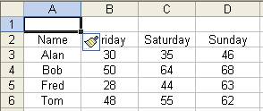
This action will add a blank row in Row 1 while all of the other information slides down. Now our screen should look like below.
What we want to do is have “Hickam’s Team Sales” appear as one cell above all of the information we have in Row 2. To achieve this goal, we must merge cells A1 through D1.
Highlight cells A1 through D1 and then go to Format on the Menu bar and choose Cells.
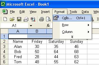
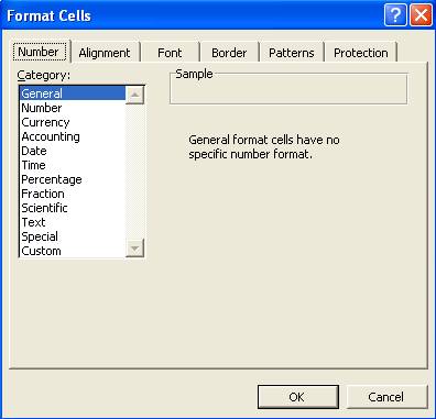
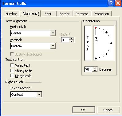
Once you choose Cells, the Format Cells screen will appear like below.
On this screen there are six tabs to choose from. The one we want to explore is the Alignment tab. So, click on the Alignment tab. The screen will now appear like below.
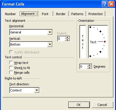
To merge the cells we have highlighted, we will check the box in front of the words “Merge Cells” which is about three fourths of the way down the screen. Once you check this box, click OK. Now the Excel screen should appear like below.
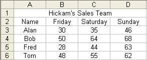
Notice that A1 through D1 is now one complete cell. Click in that cell and type in “Hickam’s Sales Team.” Center the information by clicking on
the cell again and clicking the ![]() icon.
Now your information should look like below.
icon.
Now your information should look like below.
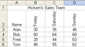
Let’s say we want to experiment with turning the days of the week on their side like below.
To do this special feature, we need to highlight B1, C1, and D1. Now go to the Menu bar and choose Format and then cells. Click on the Alignment tab. Here is our screen.
What we want to concentrate on is the right hand side of this screen that looks like below.
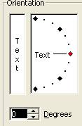
Click and hold down on the line beside the word “Text” and drag it up to the top, which will change your degrees to 90. Click OK and your information turns on its side so we now have
If you want to turn the days of the week to a 45 degree angle, highlight the cells again and go back to
the Menu bar and choose Format and then cells.
Click on the Alignment tab and either move the line to 45 degrees or
type 45 degrees in the degrees window box (![]() ). Now your document should look like
below.
). Now your document should look like
below.
Let’s look at applying some basic formulas to our data above.
Assume that we are interested in calculating the exact amount of money each person has earned over the 3-day period. For Alan, we would find his total sum by adding 30, 35, and 46, which is 111. We will do this calculation using Excel and see that this is one of the wonderful powers of Excel, for there is more than meets the eye than simply adding up these numbers, which we will soon see.
First, let’s put the wording of “Total Sales” in cell E2. Make column E wider if you have to do so. Now, we want the total sum of the sales for Alan to be in cell E3, but we do not want to simply type the number 111 in there. For this is a big no-no. What we want to do is have Excel add up cells B3, C3, and D3. The reason we do this is that if the numbers in one of these cells changes, Excel will automatically recalculate the total sum in E3. If we had typed in 111 in E3, the value would always stay 111 no matter what changed in B3, C3, or D3.
To tell Excel you want it to calculate something (add, subtract, multiply, etc.), you have to go to the cell where you want the calculation to appear and type an = sign and then what you want it to do. In this case, we will go to cell E3 and type = B3 + C3 + D3. Notice that as we type this formula in, it appears below the Menu bar in the little box titled fx.
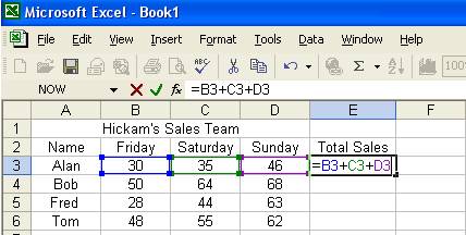
Also, notice that whenever you start with an = sign, Excel will highlight the cell location that you enter and color code the cells to match the color of the cell name. The word B3 is in blue and cell B3 has blue around the outside of the cell. It uses a different color for each cell you enter.
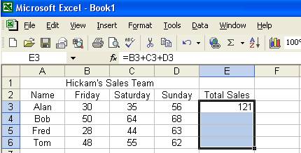
After entering =B3+C3+D3, hit the Return or Enter key and 111 appears in cell E3. Now go to cell D3 and change the value from 46 to 56. Notice that E3’s value changed from 111 to 121. Whenever any cell changes value, every cell that starts with an = sign gets recalculated. That is one of the many great powers of Excel.
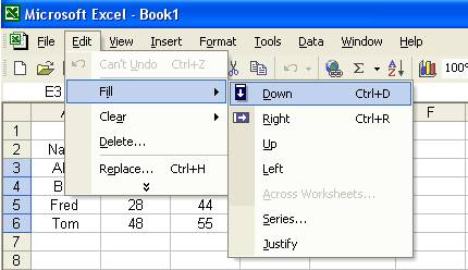
To calculate the total sales for Bob, we might go to cell E4 and enter =B4+C4+D4, and do the same thing for Fred and Tom. However, that would take a very long time if we had 500 employees. So there must be a better way or some shortcut, and there is. Since we have already entered the main formula that will apply to the other three people, all we need to do is click in cell E3 where the formula appears and hold down on the mouse button and drag down to cell E6 so that E3 through E6 are highlighted like below.
Now go to the Menu bar and choose Edit and then the Fill option. Since we are feeling the formula down, we will choose the Down selection. See below.
Now our screen appears like below with all of the information filled in.
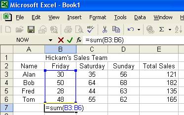
Again, go and change one of the values under Friday, Saturday, or Sunday, and you will notice that the corresponding value in column E changes. The fill right works the same way as the fill down except it fills the formula in to the right instead of down. For example, if we wanted to find the total we had in sales for Friday, we would want to add cells B3, B4, B5, and B6 and probably put this total in cell B7. So, in cell B7, put =B3 + B4 + B5 + B6 like below.
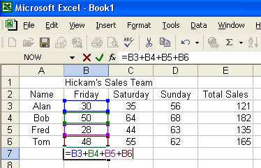
Once you hit return, 156 appears in
cell B7. Now to apply this same formula
to C7 and D7, we will not do the formula over again for each cell, but instead,
we will click in cell B7 and highlight over to cell D7 (E7 if you want to get
the grand total of sales). Again, we
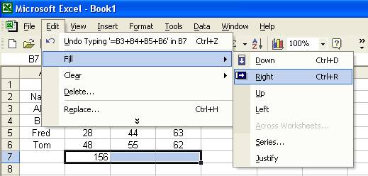
will go to the Menu bar and select Edit, Fill, and this time choose Right. (You may have to go down to the ![]() at
the bottom of the choices to make the extra selections appear.)
at
the bottom of the choices to make the extra selections appear.)
Magically the formula is filled in.
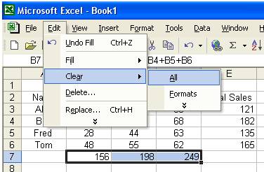
Let’s go back and erase everything in cells B7, C7, and D7. To erase a large selection of information, highlight the cells you want to erase and go to Edit on the Menu bar and choose Clear and then All.
Now all of the cells are clear of information. The reason we cleared the information is that we want to calculate the sum of the columns again, but in a somewhat quicker way. Imagine if we had 50 employees on Hickam’s Sales team. It would take forever to type in =B3 + B4 + …+ B53. So, there is a quicker way when we want to add up a lot of cells. To do this, we simply type in =sum(tell it the starting cell: tell it the ending cell). In this case we will just use the information we have and have Excel start with cell B3 and end with cell B6. So, we will click in cell B7 and enter =sum(B3:B6) This tells Excel that we want it to start with cell B3 and add through to cell B6.
After hitting Enter, B7 changes to the value of 156.
Instead of finding to the total on that day, we may want to find the average sales. Clear cell B7 by clicking in it and hitting the backspace button. The formula we will enter this time will be very similar. It will be =average(B3:B6) like below.
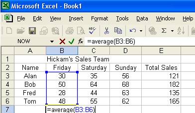
Instantly, we get the average of column B, which is 39.
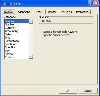
Go to cell B6 and change it from 48 to 47.99. It will change our average to 38.9975, which is not very pretty. Let’s control how that cell turns out making sure that it is always rounded to the nearest hundredth of a dollar. To control how many spaces each cell is rounded, we will click on which cell or cells we want to set, which in this case is cell B7. Now go to Format in the Menu bar and choose cells. Click on the Number tab. Our screen should now appear like below.
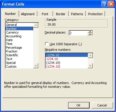
We can choose Number or Currency from the Category selection. They will do the same thing, except Currency will put a $ sign in front of your number for you. Let’s choose Number. When we do this, we get the choice of how many decimal places we want to the right of the number.
Now use the fill right button to fill in the average for the Saturday and Sunday (and Total if you like). Our final screen can be saved for future reference or for comparison of the sells for that week.
We have touched on the basics of Excel’s power. I currently use Excel for recipes, phone logs, taxes, publishing sports schedules that involve over 600 games and 75 teams, discipline records, bank deposits, grade book for the classes I teach, CPR certification of my school’s employees, and the list goes on. Never have I found a program that I have used for so many things. The next time you have a task to do that involves data of any type, think of Excel, for it is up to any challenge.